Last Sunday, we had another topic in SC03 (Non-Linear Techniques in ML). This time, it was another machine learning algorithm: Support Vector Machine, or SVM.

From what I understood at first, SVM is another type of classifier. There is also Support Vector Regression (SVR), which, as the name suggests, is the regression version.

What made this activity a little different was that we were given only 1.5 hours to understand our assigned topic and prepare something we could present to the class online.

And by “understand,” I don’t mean just reading a few slides.

We had to explain the theories and terminologies, come up with some kind of numerical, graphical, or coding demonstration, discuss practical uses, and somehow connect our topic with what the other groups were discussing.

The topics were:

• Group 1: Foundations
• Group 2: Linear SVM
• Group 3: Kernels
• Group 4: Practical SVM

Our group ended up with Practical SVM.

At first, I wasn’t sure whether that was a good thing.

“Practical SVM” sounded like it might be the easy part. Maybe we just had to show some applications, run a model, explain the results, and call it a day.

It didn’t take long before I realized that wasn’t exactly how it was going to work.

Wait, Practical SVM Means Knowing the Other Parts Too?

The problem with explaining the practical side of SVM is that you still need to understand what SVM is doing in the first place.

Before we could talk about tuning a model or evaluating one, we had to understand things like:

• hyperplanes
• margins
• support vectors
• hard and soft margins
• kernels
• C
• gamma

Basically, a good portion of what the other groups were studying.

That was when Practical SVM started to feel less like “the application part” and more like the part where everything had to come together.

We couldn’t just say, “Here is some Python code for an SVM.”

We had to understand why we were choosing certain settings and what those settings were actually doing to the model.

So while preparing our part, I started from the question that seemed most basic:

What is SVM actually trying to do?

So, What Is SVM Actually Doing?

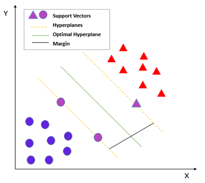
The way I started making sense of SVM was to think about two groups of points on a graph.

Let’s say one group is blue and the other is red.

If the two groups can be separated, we could draw a line between them and use that line to decide where a new point belongs.

In SVM, that decision boundary is called a hyperplane.

There might be several lines that can separate the two groups, though. SVM isn’t just looking for any line that works.

It tries to find a boundary with the largest possible space between the two classes.

That space is the margin.

Source: “Linear SVM components” on ResearchGate

Then there are the support vectors, which are the points closest to the decision boundary.

Those points are especially important because they help determine where the boundary ends up.

That was probably the first point where the name Support Vector Machine started to make a little more sense to me.

The points near the boundary are the ones “supporting” where that boundary gets placed.

For a linear SVM, the hyperplane is commonly represented as:

w·x + b = 0

In two dimensions, we can just imagine it as a line.

Once the number of features starts increasing, visualizing it becomes harder, but the idea is still the same: SVM is trying to find a boundary between classes.

Perfect Separation Sounds Nice… Until Real Data Shows Up

Then we got into hard margin and soft margin.

A hard-margin SVM basically wants perfect separation.

No mistakes.

Every point should be on the correct side of the boundary.

That sounds great until you remember that real-world datasets tend to be messy.

There can be noise. There can be outliers. Two classes can overlap. One unusual observation might be sitting in a place where it doesn’t seem to belong.

If the model insists on classifying every single training point correctly, it can end up fitting itself too closely around those unusual cases.

That’s where the soft margin comes in.

Instead of demanding perfection, a soft-margin SVM allows some violations or even some misclassified points if that produces a boundary that generalizes better.

I liked this idea because it connects to something that keeps appearing in machine learning:

A model doing perfectly on the training data isn’t necessarily a good thing.

Sometimes a few mistakes are acceptable if the model works better on data it hasn’t seen before.

And this is where another letter enters the picture.

C.

Then We Met C

C was probably one of the parameters I had to stop and think about for a while.

The way I eventually understood it was that C controls how forgiving SVM is about mistakes.

With a smaller C, the model is more willing to tolerate some violations.

It’s almost like saying:

“A few mistakes are fine. Just try to keep the boundary reasonably simple.”

That can result in a wider margin, but if C becomes too small, the model might become too relaxed and start underfitting.

A larger C does the opposite.

Now the model becomes much less forgiving.

It’s more like:

“Try harder not to misclassify these training points.”

That can make the model fit the training data more closely, but if C is too large, we risk making the decision boundary too specific to the training data.

So C isn’t a “higher is better” kind of setting.

It’s a trade-off.

And then, just as C started to make sense, kernels and gamma entered the picture.

Kernels, Gamma, and the Non-Linear Part

A straight line is nice when the data can actually be separated with a straight line.

But sometimes it can’t.

This is where the kernel comes in.

Our presentation included three common ones:

• Linear
• Polynomial
• RBF

The linear kernel makes sense when the data can be separated using a linear boundary.

The polynomial kernel can represent more complicated curved boundaries.

Then there’s the RBF kernel, which gives SVM more flexibility when dealing with non-linear patterns.

This part connected directly with the group assigned to Kernels.

Their topic was about how kernels work.

For our Practical SVM topic, the question became slightly different:

Okay, now that we have these kernels, which one are we actually supposed to use?

And the answer wasn’t simply, “RBF is better,” or “Always use linear.”

We would need to test different options and see which configuration works better for the data.

With RBF, we also get another parameter to think about: gamma.

Gamma was another one that sounded confusing until I found a simpler way to think about it.

If C is about how much the model cares about mistakes, gamma is more about how far the influence of each training point reaches.

A low gamma means a point can influence a relatively large area.

A high gamma means that influence becomes much more local.

With very high gamma, the model can start creating extremely specific regions around the training points, which can lead to overfitting.

So now we had C, gamma, and different kernels.

At this point it became pretty obvious to us why we needed some systematic way of testing all these combinations instead of just picking numbers because they looked reasonable.

Turning All of That Into Something We Could Actually Run

This was where our Practical SVM workflow started to make much more sense.

We summarized it as:

1. Split the data
2. Scale the features
3. Choose the search space
4. Cross-validate
5. Evaluate

That looks simple when written in one line.

But each step exists for a reason.

Split the Data

First, we keep a portion of the dataset aside as a final test set.

The important part here is that we don’t keep looking at the test set while making decisions about the model.

It’s supposed to represent data the model hasn’t seen.

Scale the Features

This part is especially important for SVM because it depends on distances and dot products.

Imagine having two features:

Feature	Typical Range
Age	18–80
Annual income	₱100,000–₱5,000,000

Those numbers are on completely different scales.

Without scaling, income could dominate the calculations simply because its values are much larger.

It doesn’t necessarily mean income is actually more important. The numbers are just bigger.

So we scale the features first.

One detail we also had to remember was to fit the scaler using the training data only.

Otherwise, information from the test set could leak into the training process.

Choose What We Want to Test

Then we decide which combinations we want to try.

Which kernel?

What values of C?

If we’re using RBF, what values of gamma?

This is basically our search space.

Cross-Validate

Instead of testing all these combinations against our final test set, we use cross-validation on the training data.

The training data gets divided into different portions so that candidate models can be trained and validated several times.

This gives us a better way of comparing settings without repeatedly touching our final test set.

Evaluate

Once we’ve selected a configuration, we finally evaluate the model on the test data.

This was also where I was reminded that simply looking at accuracy isn’t always enough.

Accuracy Isn’t the Whole Story

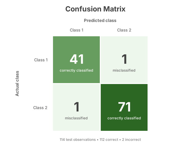
Our presentation used a confusion matrix as the starting point for evaluating the classifier.

From there, we can look at metrics such as:

• Accuracy
• Precision
• Recall
• F1-score
• ROC-AUC

I had already encountered some of these before, but seeing them as part of an actual model workflow made their purpose clearer.

Accuracy answers the straightforward question:

How many predictions were correct overall?

But precision and recall let us look at the mistakes more carefully.

Precision asks how many of the observations predicted as positive were actually positive.

Recall asks how many of the actual positive observations the model successfully found.

Then F1-score tries to balance precision and recall.

So depending on the problem, two models with similar accuracy could still behave very differently.

That brings us to the part where all of this finally turned into something we could actually run.

The Demo

For our demo, we used our favorite dataset (we’ve been using this dataset from the other courses 😀): Breast Cancer Wisconsin dataset.

It has 569 observations and 30 numeric features.

For the experiment, we used:

• an 80/20 stratified train-test split
• 5-fold cross-validation
• F1-score as the metric for searching through the candidate configurations

After the search, the selected settings were:

Parameter	Selected Value
Kernel	RBF
C	10
Gamma	0.01

The final model achieved:

• 98.2% accuracy
• 98.1% macro F1-score

And the confusion matrix looked like this:

This was probably the part that helped everything come together for me.

Seeing 98.2% accuracy is nice, but looking at the confusion matrix makes that number much more concrete.

There were 114 observations in the test set, and only two were classified incorrectly.

More importantly, I could now connect those results back to everything we had just studied as a group.

We didn’t simply call an SVM function and magically get 98.2%.

We had to scale the features.

We had to decide which parameters to test.

We had to compare kernels.

We had to tune C and gamma.

We had to use cross-validation.

And only after all of that did we evaluate the final model.

That’s when “Practical SVM” finally started feeling like the right name for our topic.

So, Is SVM Always a Good Choice?

Of course, after spending all that time learning SVM, it would be tempting to think we should use it everywhere.

Not exactly.

From our presentation, some of SVM’s strengths are that it can work well in high-dimensional spaces, handle non-linear boundaries through kernels, and perform well with small-to-medium-sized datasets.

But there are trade-offs too.

It’s sensitive to feature scaling.

Training can become slow when the dataset gets very large.

There are several settings to tune.

And compared with simpler models, explaining exactly why an SVM made a particular prediction can be more difficult.

So, like most things I’ve encountered so far in machine learning, it isn’t really about finding one algorithm that beats everything else.

It’s about understanding when a particular algorithm makes sense.

Maybe the Time Limit Was the Point

One thing I haven’t mentioned much is that I actually have this small fear of timed learning activities.

Being told, “You have 1.5 hours to learn this topic and present it afterward” immediately puts some pressure on me.

And since this was a remote class, 1.5 hours doesn’t always mean you actually get the entire 1.5 hours.

Anything can happen at home.

Someone might call you. You might need to step away for a few minutes. The internet could suddenly decide that this is the perfect time to stop cooperating. Even a small interruption feels much bigger when you know there’s a timer running somewhere in the background.

So when the activity started, part of me was already thinking about the time.

What if we don’t understand the topic fast enough?

What if we spend too much time on one concept?

What if something interrupts us halfway through?

But after going through the activity, I also started appreciating the other side of it.

Having a limited amount of time somehow forces you to learn.

There’s no “I’ll read this later” or “I’ll come back to this part eventually.” We knew that after 1.5 hours, we had to present something. That meant we had to focus on what mattered, ask questions when something didn’t make sense, divide the work, and try to build a reasonable understanding within the time we had.

It actually reminded me a little of the Pomodoro technique.

I sometimes find it easier to focus when there’s a clear block of time dedicated to one thing. Instead of thinking about how much there is to learn, the goal becomes simpler:

For this amount of time, this is what I’m working on.

Of course, 1.5 hours of studying SVM with a presentation waiting at the end is a little more intense than a normal Pomodoro session.

But I think the idea is similar.

The time limit creates some pressure, but it also creates a boundary. For that period, we weren’t expected to become experts on SVM. We just had to learn as much as we reasonably could, make sense of it, and explain what we understood.

And maybe that’s something I need to get more comfortable with.

Learning doesn’t always have to happen when I have an entire free afternoon, the perfect environment, and enough time to understand everything.

Sometimes you get 90 minutes.

Sometimes you get interrupted.

Sometimes you finish the session still having questions.

But you can still come out of it understanding more than you did when the timer started.

For this class, that happened to be SVM.

And considering that we started with a topic we still had to unpack and ended the session presenting a working example of it, I’d say those 90 minutes weren’t wasted.