So, What Does K Mean?
As previously mentioned in my article, I was starting my journey from the ground up with Machine Learning. In parallel, I’m also taking up the Non-Linear Techniques (SC03) course with the same instructor, currently in my second year.
Yesterday was our first day in class, and I wanted to log and document the topics being taught here since writing about them is one of the ways I recall what I learned.
Our instructor started with a recap of Machine Learning, the linear techniques we previously discussed, and how those ideas continue into the current course.
Previously, we’ve been dealing with inputs and outputs that are expected to have linear relationships. This time, we’re moving into techniques that can handle relationships that aren’t necessarily linear.
One idea that keeps coming back is that Machine Learning is really about finding patterns in data.
Sometimes, we already know the answer we want the machine to learn. Other times, we simply give it the data and let it discover useful structure on its own.
That brings us to the first learning algorithm for this course: K-means.
K-Means
K-means is a clustering algorithm under unsupervised learning.
The K in K-means represents the number of clusters, or groups, that we want the algorithm to divide our data into. It’s like group chats, but for data.
Unlike supervised learning, there are no labels telling the model what each data point is supposed to be. Instead, the algorithm looks at the data and tries to group together points that are close to one another.
In a way, the machine is learning through observation.
To perform K-means, the steps are:
- Determine the value of K.
- Select K random data points from the dataset.
- Assign the other data points to the nearest K point.
- Determine the mean of each cluster and use those means as the new K points.
- Check whether new assignments are encountered. If yes, go back to Step 3. Otherwise, the clustering process is done.
Let’s try to work through an example.
Example Dataset
Dataset:
1, 2, 4, 5, 16, 17, 18, 19, 23, 24, 25, 26
First, we choose the number of clusters.
K = 3
This means we are dividing the dataset into three groups:
K1
K2
K3
Next, we randomly select three data points from the dataset to serve as our initial cluster centers, also called centroids.
K1 = 2
K2 = 5
K3 = 18
With the three starting points selected, the next step is to assign every number in the dataset to the nearest centroid.
Using:
K1 = 2
K2 = 5
K3 = 18
we end up with the following clusters:
K1 = 2  -> {1, 2}
K2 = 5  -> {4, 5}
K3 = 18 -> {16, 17, 18, 19, 23, 24, 25, 26}
Basically, every data point looks at K1, K2, and K3 and asks:
Which one am I closest to?
Then it joins that group.
This is probably where the “group chat” analogy started making more sense to me. The data points are basically finding the group they fit into best based on distance.
Finding the New Center of Each Group
Now that the members of each cluster have been identified, we calculate their means.
These means become the new centroids.
For K1:
(1 + 2) / 2 = 1.5
So:
K1 = 1.5
For K2:
(4 + 5) / 2 = 4.5
So:
K2 = 4.5
And for K3:
(16 + 17 + 18 + 19 + 23 + 24 + 25 + 26) / 8 = 21
So:
K3 = 21
Our centroids have now moved from:
2, 5, 18
to:
1.5, 4.5, 21
Since the values of the centroids changed, the algorithm isn’t done yet.
We have to go back and assign the data points to their nearest centroid again.
This repeating process — assigning points, calculating the mean, moving the centroid, and assigning the points again — is really the heart of K-means.
And We Go Again…
Using the new centroids:
K1 = 1.5
K2 = 4.5
K3 = 21
we repeat the assignment process.
Interestingly, the clusters remain the same:
K1 = 1.5 -> {1, 2}
K2 = 4.5 -> {4, 5}
K3 = 21  -> {16, 17, 18, 19, 23, 24, 25, 26}
When we calculate their means again, we still get:
K1 = 1.5
K2 = 4.5
K3 = 21
Nothing moved this time.
And that’s our stopping point.
The clusters are no longer changing, which means the algorithm has reached its final grouping.
At first, I thought K-means would involve some complicated computation happening all at once. But seeing it manually made it much easier to understand.
It’s really an iterative process:
group -> average -> move -> regroup -> repeat
until nothing changes anymore.
But Are These Actually the Best Clusters?
There’s one slight problem.
Remember that our initial centroids were chosen randomly.
We started with 2, 5, and 18, but another run could have started with completely different points. Different starting points could potentially lead to a different clustering result.
So how do we know which clustering result is better?
This is where variance comes in.
Variance, in this context, gives us an idea of how spread out the values inside each cluster are.
If the members of a cluster are relatively close to one another, the variance is lower. If they’re scattered farther apart, the variance becomes higher.
We calculate the sample variance of each cluster using:
Here, xᵢ is each value in the cluster, x̄ is the cluster mean, and n is the number of values in that cluster.
For the clusters in our example, the lecture calculated the following:
K1 variance = 0.5
K2 variance = 0.5
K3 variance = 15.43
Giving us a:
Total variance = 16.43
The idea taught in class was to perform the clustering several times and compare the results.
Since the initial K points are randomly selected, we can end up with different cluster arrangements. Among those attempts, we prefer the clustering with the lowest variance.
In simple terms: we want groups whose members actually stay reasonably close together.
It reminds me of splitting people into group chats. You could randomly put everyone together, but a better grouping would have people inside each chat who have more in common with one another.
Okay, but Who Decided That K Should Be 3?
There is still another question hiding in our example.
We were simply given:
K = 3
But with a new dataset, how would we know whether we should create 2 clusters? 3? 4? 10?
Picking too few clusters might put very different data points together.
On the other hand, continuously increasing K would reduce the variance because we’re creating smaller and smaller groups. In the extreme case, if every data point had its own cluster, there wouldn’t be much point in clustering at all.
This is where the Elbow Method enters the conversation.
The Elbow Method
The process starts by trying different values of K.
For every K, we determine the best clusters and record their variance.
We can then plot them on a graph:
- the x-axis represents the value of K;
- the y-axis represents the variance.
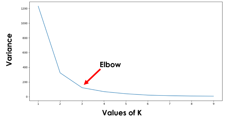
Variance usually drops sharply for the first few values of K.
Eventually, however, increasing K only gives us smaller and smaller improvements.
The point where that decrease starts noticeably slowing down looks somewhat like an elbow on the graph.
Hence, creatively enough, the Elbow Method.
That elbow becomes our candidate for the best value of K.
In the example graph shown in class, the elbow appears around K = 3. After that point, increasing K continues to reduce variance, but the improvement becomes much less significant.
My Takeaway
What I liked about K-means as an introduction to unsupervised learning is that it makes the idea of a machine “finding patterns” much more concrete.
Nobody tells the model:
“1 and 2 belong together.”
Nobody labels 16, 17, and 18 as one category.
Instead, we give it the data, tell it approximately how many groups we’re looking for, and let distance and repetition reveal the structure.
That also made the difference between supervised and unsupervised learning click a little more for me.
With supervised learning, there’s usually an answer we already know and want the model to learn how to predict.
With K-means, there isn’t necessarily an answer key.
We’re essentially asking:
“Here’s a bunch of data. Do you notice any natural groups in here?”
And K-means responds by repeatedly moving things around until the group chats finally stop changing.
For my first algorithm in Non-Linear Techniques, I’d say that’s a pretty neat place to start.